リム傑威
Lim Jackwee
THEORY NMR
NMR commands for Topspin Bruker Program
1. rpar: reads in the list of expts to choose from
2. lockdisp: opens lock display window (lower signal to 80% during zg or multizg)
3. getprosol: reads the probehead and solvent dependent parameter
4. ased: edits the acquisition parameters used in the current pulse program
5. eda/edc: edits/copies acquisition parameters
6. edasp: sets up nuclei and spectrometer routing
7. edte: sets up temp control
8. wobb: manual tuning and matching of the probehead
9. atma/atmm: automatic/ manual tuning and matching of ATM probeheads
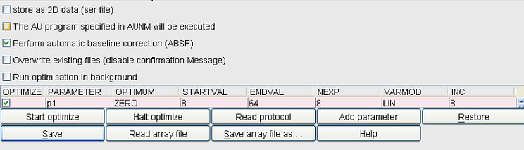
10. popt: parameter optimization
11. wsh: writes a set of shim values
12. rsh: reads shim file
13. zg/ multizg: initiates experiment(s)
Steps (short): Data acquisition
1. Use depth gauge in spinner turbine to measure sample height
2. In Topspin window, click lift to leave gas (Feel the gas with hand over the top of the magnet, if not ALERT!!!)
3. Click 'lift' to lower NMR tube (Green Light Down appears)
4. 'rpar' to read in pulse program
5. 'getprosol' to load probe dependent parameters
6. 'lock' (select solvent e.g H2O+D2O)
7. 'atma' to invoke automatic tuning (wait for finished message)
8. 'topshim' to invoke automatic shimming (wait for finished message)
9. 'rga' to invoke receiver gain adjustment
10. 'd1' to invoke delay between pulse e.g 1 (1-4s)
11. 'popt' to vary p1 values from 90˚ (10-20us) to 360˚ pulse (used to monitor water suppression at 4.7ppm in 1D mode especially for nD expts)
12. Click start optimize in popt panel to note maximal methyl peak and minimal water peak at p1
13. Use this p1 in nD pulse program and update others e.g. DS, NS, SW, RG etc
14. 'rga' and lower rga if receiver gain overflow(or recheck p1to suppress water peak)
15. 'zg' to start acquisition
Steps (short): Data Processing
1. ef or efp
e comes from em = for exponential multiplication set by lb command for line broadening (usually lb = .5Hz for proton and lb = 10 HZ for carbon). f comes from ft = for Fourier transformation of time domain data to frequency domain. p comes from pk = for phase correction using the last applied phase
2. apk for automatic phasing
Source: http://triton.iqfr.csic.es/guide/man/
Bruker Command Manual at http://www.calstatela.edu/sites/default/files/dept/chem/nmr/pdf-forrms/avance-ii-400-mhz-bruker_manual.pdf
1H 90˚ calibration Manual at http://web.mit.edu/speclab/www/PDF/DCIF-90pulse-Bruker-j07.pdf
Diagrammatic Representation of Rotations


The rotation of an operator  gives two terms:
1. Â multiplied by the cosine of an angle
2. The new operator, B multiplied by the sine of the same angle
Thus the effect of any rotation is
cosθ * Â + sinθ * B
e.g. for θ, angle πJ12τ = π/2 when τ is 1/(2J12) will complete the B operator since cos90˚ = 0 and sin90˚ = 1
Operators for two spins
Description operator(s)
z-magnetization on spin 1 Î1z
in-phase x- and in-phase y-magnetization on spin 1 Î1x, Î1y
z-magnetization on spin 2 Î2z
in-phase x- and in-phase y-magnetization on spin 2 Î2x, Î2y
anti-phase x- and anti-phase y-magnetization on spin 1 2Î1xÎ2z, 2Î1yÎ2z
anti-phase x- and anti-phase y-magnetization on spin 2 2Î1zÎ2x, 2Î1zÎ2y
multiple-quantum coherence 2Î1xÎ2x, 2Î1xÎ2y, 2Î1yÎ2x, 2Î1yÎ2y
non-equilibrium population 2Î1zÎ2z
Coupling constants in Hz
Example for in-phase along x (Î1x) to in-phase along -x (-Î1x)
(a) (b) (c) (d) (e)
Î1z --->Î1x ---> cos(πJ12τ)Î1x + sin(πJ12τ) 2Î1yÎ2z --->2Î1yÎ2z --->cos(πJ12τ)2Î1yÎ2z - sin(πJ12τ)Î1x --->-Î1x
(a) 90˚ pulse along y-axis on spin 1 in z-equilibrium to rotate onto x-axis
(b) Hamiltonian coupling: πJ122Î1zÎ2z and angle is πJ12τ for time τ on Î1x
πJ12τ2Î1zÎ2z during free Hamiltonian evolution of Î1x for Hamiltonian (πJ122Î1zÎ2z) * time τ
In-phase term Î1x goes into anti-phase 2Î1yÎ2z in the presence of Hamiltonian coupling term 2Î1zÎ2z
(c) complete conversion to anti-phase when τ is 1/(2J12)
(d) Hamiltonian evolution of 2Î1yÎ2z for time τ: πJ12τ2Î1zÎ2z
(e) complete conversion to in-phase when τ is 1/(2J12) to in-phase along -x, starting from in-phase along x in (b)
Example for coherence transfer
2Î1yÎ2z --->2Î1zÎ2z --->-2Î1zÎ2y
(a) (π/2)Î1x on spin 1
(a) (π/2)Î2x on spin 2
Only anti-phase terms are transferred during complete coherence transfer (when the in-phase cos(π/2) term = 0, see Heteronuclear coherence transfer by INEPT below)
(a) (b)
Example for spin echo for one spin

Î1x --->cos(Ωτ)Î1x + sin(Ωτ)Î1y --->cos(Ωτ)Î1x - sin(Ωτ)Î1y --->cos(Ωτ)cos(Ωτ)Î1x + sin(Ωτ)cos(Ωτ)Î1y - cos(Ωτ)sin(Ωτ)Î1y + sin(Ωτ)sin(Ωτ)Î1x == Î1x
(a) ΩτÎ1z during free Hamiltonian evolution of Hamiltonian (ΩÎ1z) * time τ on Î1x
(b) πÎx :180 about x does not affect Î1x and inverts Î1y
(c) ΩτÎ1z : 2nd delay echoes back to Î1x (U-turn)
Hence τ--π--τ == π
(a) (b) (c)
cancels out
Example for spin echo for Homonuclear coupled spin
Î1x ---> ---> cos(2πJ12τ)Î1x + sin(2πJ12τ) 2Î1yÎ2z
(a) Spin-echo is an outcome of π and 2τ independent of offset.
Hamiltonian coupling: πJ122Î1zÎ2z. But angle is 2πJ12τ for time 2τ on Î1x
Overall 2πJ12τ2Î1zÎ2z during free Hamiltonian evolution of Hamiltonian (πJ122Î1zÎ2z) * time 2τ on coupled Î1x
In-phase term Î1x goes into anti-phase 2Î1yÎ2z in the presence of Hamiltonian coupling term 2Î1zÎ2z
Thus in homonuclear systems, spin echoes allow the coupling to evolve while suppressing evolution due to offset. In heteronuclear systems, spin echoes can suppress evolution of heteronuclear couplings or invoke decoupling.
(a)
Example for Heteronuclear coherence transfer by INEPT
Starting with Îx for the first echo,
Îx ---> cos(2πJISτ1)Îx + sin(2πJISτ1)2ÎySz --->-sin(2πJISτ1)2ÎzSy ---> sin(2πJISτ2)sin(2πJISτ1)Sx
(a) 1st spin echo τ1--π--τ1 results the in-phase term Îx to go into anti-phase 2ÎySz (see homonuclear coupled spin, above)
(b) Coherence transfer, (π/2)Îx, (π/2)Sx only affect the anti-phase 2ÎySz term
Only anti-phase 2ÎySz terms are transferred to give anti-phase -2ÎzSy due to complete coherence transfer (since in-phase cos(π/2)Îx = 0 when τ1 = 1/(4JIS))
(see Diagrammatic Representation of Rotations: cosθ * Â + sinθ * B and coherence transfer)
For the 2nd echo,
(c) 2nd spin echo τ2--π--τ2 results the anti-phase term -2ÎzSy to return to in-phase Sx in the presence of Hamiltonian coupling
Maximum transfer when τ1 = 1/(4JIS) and τ2 = 1/(4JIS)
(a) (b) (c)
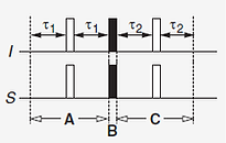
Example for Heteronuclear coherence transfer using HMQC
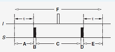
Starting with Îx
Îx ---> cos(πJISτ)Îx + sin(πJISτ)2ÎySz --->-sin(πJISτ)2ÎySy --->-cos(Ωst)sin(πJISτ)2ÎySy + sin(Ωst)sin(πJISτ)2ÎySx --->-cos(Ωst)sin(πJISτ)2ÎySz --->cos(Ωst)sin(πJISτ)sin(πJISτ)Ix
(a) Hamiltonian coupling: πJ122Î1zSz and angle is πJ12τ for time τ on Îx
(b) S-spin 90˚ heteronuclear complete coherence transfer (π/2)Sx of only anti-phase term 2ÎySz to give multiple quantum coherence -2ÎySy
(c) Evolution under only one S-spin offset for period C: ΩstSz (I-spin offset is refocused due to 180˚ central pulse during period F)
(d) 90˚ pulse to S, (π/2)Sx transfers only the first term -2ÎySy to give -2ÎySz (since there is no effect on 2ÎySx)
(e) Hamiltonian coupling: πJ122Î1zSz and angle is πJ12τ for time τ on -2ÎySz returns to in-phase Ix
(a) (b) (c) (d) (e)
Period C: one S-spin Hamiltonian evolution ΩstSz
Weak Signal and Line-Broadening in NMR
The linewidth of a peak resonance is determined by the lifetime of the magnetic states between which NMR transition occurs. The lifetime of the states can be related to the linewidth by the Heisenberg uncertainty principle. The Heisenberg uncertainty principle relates how precisely we can define the momentum and position of a particle at the same time thus the shorter the lifetime, the less certainty we can define its energy.
For example, a magnetic nucleus in a ground state wtih long lifetime goes to an excited state with short lifetime, Δt. The uncertainty principle tells us that the excited state cannot be precisely defined or have low probability of being in the excited state. The transition energy ΔΔE and its precision of the transition frequency Δv are related by,
ΔΔE ~ h/2π * 1/Δt ~ ħΔv

The shorter liftetime of the excited state is possible by increased relaxation processes by a number of ways e.g. presence of paramagnetic metal ions and increased viscosity. When relaxation is fast, the NMR lines are broad. Next two major relaxation processes in NMR are discussed.
Source: https://www.chem.wisc.edu/areas/reich/nmr/08-tech-01-relax.htm
1. Spin-lattice (T1 relaxation)
T1 is responsible for loss of signal intensity
The excited nuclei in the sample or the sample lattice is surrounded with other nuclei in vibrational and rotational motions. The effect from the mobile lattice creates a magnetic field called the lattice field which can interact with the excited nuclei, causing it to lose energy (or return to the ground state). The relaxation time, T1 or the average lifetime of the excited nuclei depends on its gyromagnetic ratio and the lattice mobility. As the mobility of lattice decreases, the probability of the lattic interacting with the excited nuclei also decreases (or inefficient T1 relaxation). However, at extreme mobility, the probability of the lattice interacting with the excited nuclei can also decrease (also inefficient T1 relaxation).
The actual efficiency of T1 relaxation is optimal when the molecular motion is at the Larmour precession frequency. At room temperature, mobile liquid is moving several magnitude orders higher than ν0, thus has inefficient T1 relaxation (longer T1 relaxation time). For larger molecule, molecular motion is slower, more efficient T1 relaxation and thus shorter T1 relaxation time. However, at some point, the average molecular motions become slower than ν0, resulting in longer T1 relaxation time as observed for τc ~ ns in proteins.
2. Spin-spin relaxation (T2 relaxation)
T2 is more responsible for linewidth broadening than T1
The excited nuclei can interact with neighboring nuclei with identical precession frequency but different quantum states. Although there is no net change in the population in the ground and excited energy states, the average lifetime of the excited nuclei decreases thus resulting in linewidth broadening. Hence an excited nuclei surrounded by more neighboring nuclei due to more possible T2 spin-spin relaxation (shorter lifetime = more uncertainty) will result in severe linewidth broadening.
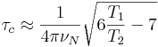
Rotational correlation time in NMR
The rotational correlation time (τc) defines the Brownian rotation diffusion time of a particle in solution.
For rigid protein molecule (< 25kDa), in the limit of slow τc >> 0.5ns and high magnetic field >> 500MHz, τc is related to T1/T2 15N relaxation by
Protein MW (kDa) 15N T1 (ms) 15N T2 (ms) τc(ns)
Ubiquitin 9.0 441.8 144.6 4.40
DvR115G 10.9 608.7 115.6 6.50
SoR190 13.8 697.5 100.9 7.70
ER540 18.8 909.0 66.5 11.30
MvR76 20.2 1015.0 64.5 12.20
Data from 600MHz at 298K
Here we see that as the molecular weight increases, the T1 increases due to longer time spent to return to equilibrium within the lattice (inefficient T1 relaxation for τc ~ns, where motion is slower than ν0), and T2 decreases due to more spin-spin relaxation involving more neighboring nuclei.
Source: http://www.nmr2.buffalo.edu/nesg.wiki/NMR_determined_Rotational_correlation_time